6  IRF Calibration

The instrument response function (IRF) describes the detection system’s response to an ultrashort light pulse. Its timing relative to a measured decay affects reconvolution fitting and IRF-based phasor calibration. This chapter covers estimating and confirming that shift in Data Extraction → Numerical.

6.1 When this stage is needed

An IRF shift is required when at least one channel meets either of these conditions:

Channel input and selected extractor	How its shift is determined
Raw FLIM with Lifetime fit selected	Fit calibration optimizes the shift during reconvolution fitting. This is required even when phasor features use a calibration dye.
Raw or pre-fitted FLIM with Lifetime fit free selected and calibration method set to IRF	Fit-free IRF calibration estimates the shift by cross-correlation. If raw lifetime fitting is also selected, its fitted shift is reused.

The app evaluates these conditions separately for each channel. Estimate and confirm shifts for the channels that meet them. Each required channel appears in its own initially open shift calibration expander, which can be collapsed after inspection. Then continue to Numerical Feature Extraction.

A calibration dye is a Fluorescence Lifetime Standard: its reference-based phasor calibration runs during fit-free feature extraction. It does not trigger this IRF shift stage. A workflow with only intensity-only channels also proceeds directly to extraction. QPI background correction has its own per-channel calibration in the same Numerical workflow.

6.2 Input

Open Data Extraction → Numerical, select the source folder, and review its file and acquisition checks. Click Start calibration. The app automatically saves the metadata, then presents the calibration controls. For FLIM channels, review the fitting options and click Optimize for Shifts; this button reads Calibrate channels when QPI background correction is also required.

6.3 Fit Calibration

The IRF can shift relative to the measured decay between experiments. For a raw FLIM channel with Lifetime fit selected, estimate and confirm its IRF shift before reconvolution fitting. Pre-fitted lifetime values are read directly and do not enter this fitting-based shift search.

It is performed in two steps:

1. Gather the high signal-to-noise ratio (SNR) decay curves
2. For each curve, perform reconvolution fitting and set the shift value as the free parameter to be optimized/fitted. The shift search range is centered on the initial shift guess and extends \(\pm 2 \times \text{FWHM}\) of the IRF in both directions, where FWHM is the full width at half maximum of the IRF measured in time bins. This focused search window prevents the optimizer from getting stuck in suboptimal basins when time gates are restrictive.

The distribution of the shift values is displayed as an interactive scatter plot. When clicking on a point, the corresponding decay curve with the fitted curve and the key statistics are displayed for diagnostics. Based on the distribution or using certain prior knowledge, users can specify the shift value applied to all fields of view (if Fix the Shift is selected, see fitting options), or use the fov-specific shift value found by the fitting (if Fix the Shift is deselected).

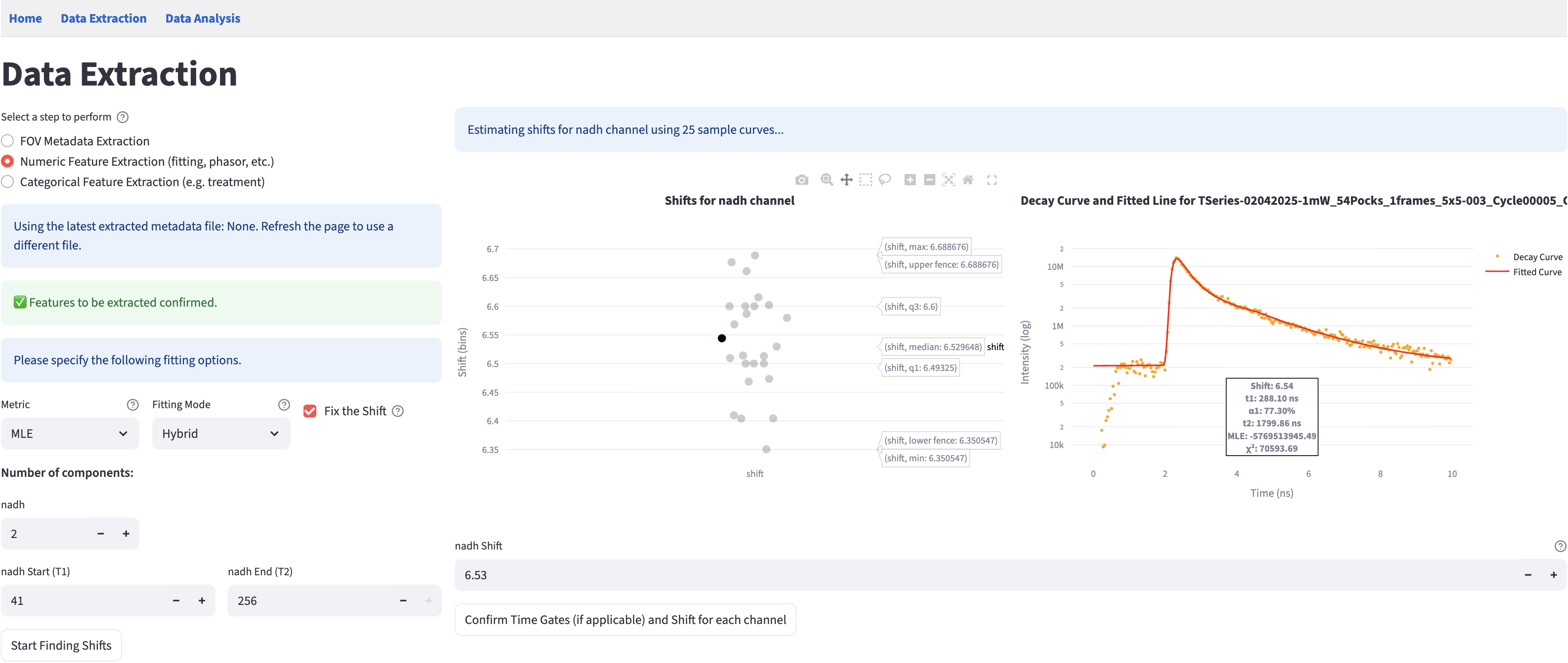
Shift calibration using the 3d_decay_1channel example: 25 NADH fields of view, with Mosaic16 selected and the full 0–256 time gate.

6.3.1 Gather High SNR Decay Curves

The high-SNR curves are gathered according to the decay type. For 2D input, the selection targets approximately 30 curves, with at least one per FOV (one CSV file). It prefers the brightest curves below 100000 photons; if a FOV has none below that threshold, it uses its brightest curves without the cap. For 3D/4D input, one curve per image sums the pixels inside its ROI mask.

6.3.2 Reconvolution Fitting

Fitting is essentially an optimization problem: it minimizes the difference between the fitted curve and the measured curve. The fitted curve is modeled by an \(n^{th}\) component exponential function convolved with the shifted IRF, and the difference is modeled as an objective metric. Therefore, users are provided with controls over two parts of the fitting process through the fitting options panel:

1. How to construct the objective metric
2. How to perform the optimization

Implementation-wise, FLIM Playground uses the lmfit package that takes generic objectives to perform the optimization process that is flexible enough to handle the reconvolution fitting.

Each decay curve is fitted independently. Fit calibration (one optimization per high-SNR curve in the IRF shift step) and Lifetime fit ROI-level extraction (one optimization per ROI per channel) both schedule those independent fits in parallel across CPU cores, so on a multi-core machine many fits run at once.

The fitting-options panel appears when a channel uses raw Lifetime fit and shifts still need estimation.

Fitting controls combine the objective and per-channel model settings.

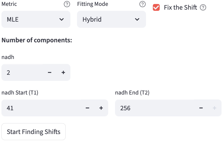
Let’s break down the fitting options one by one.

Number of Components

The number \(n\) in the \(n^{th}\) component exponential function: \[ I(\mathbf{t})=\sum_{i=1}^{n} A_i\, e^{-\mathbf{t}/\tau_i}, \qquad \tau_i>0 \]

Therefore, \(n\) determines the parameters to be fitted: the amplitudes \(A_i\) and the lifetimes \(\tau_i\). \(\mathbf{t}\) is the time axis of the decay curve calculated by the duration and time bins from the decay info: \[\mathbf{t}=\bigl[0,\ \Delta t,\ 2\Delta t,\ \ldots,\ (N-1)\Delta t\bigr], \quad \text{where }\Delta t=\frac{T}{N}. \]

It supports \(n=1,2,3\) components.

Additionally, the constant offset parameter (\(Z\)) that represents a time-independent background (i.e., room light) is also optimized¹.

\[ \hat{y}(t) = \bigl[I(t) + Z\bigr] \circledast \text{IRF}(t) \]

where \(\circledast\) denotes circular (periodic) convolution, implemented by multiplying the FFTs of the decay and IRF, then applying the inverse FFT. Circular convolution correctly accounts for the wrap-around effects inherent in periodic TCSPC decays, where photons arriving after the end of the measurement window appear at the beginning of the next period.

NotePrevious Versions (< 1.8.0)

In versions prior to 1.8.0, the fitting process utilized linear convolution with a cut off:

\[ \hat{y}(t) = \bigl( I(t) * \text{IRF}(t) \bigr)_{0:N} + Z \]

where \(*\) denotes linear convolution and the subscript \((0:N)\) denotes truncating the result to the length of the original decay curve, effectively ignoring the part of the convolution that extends beyond the measurement window. The difference between this approach and circular convolution is minimal for shorter lifetimes. However, the correct way to fit incomplete decays is formulated above using circular convolution, which is now the standard used in the latest version.

Fixed Lifetimes

While finding the optimal amplitudes \(A_i\) and lifetimes \(\tau_i\) (when number of components is greater than 1), users can optionally assign fixed values to specific \(\tau_i\) components during the interactive fitting phase. These explicit constraints remain constant (are not treated as free parameters) while minimizing the cost metric, making the optimization more robust when the true lifetime state is known. The default fixed lifetime values can be initialized in the Data Extraction Configuration.

Note

Fixed lifetimes apply only to channels that FLIM Playground fits. For pre-fit inputs (SPCImage .asc), whose lifetimes are read rather than fit, the fixed-lifetime controls are not shown.

Time Gates

Detector dead time can make some bins at the beginning or end of a decay unreliable. Set Start (T1) and End (T2) independently for each fitted channel to choose the bins included in its fitting objective. T1 is included and T2 is excluded: the default 0–256 uses bins 0–255 of a 256-bin decay.

To adjust the gates in the 3d_decay_1channel example:

1. Select a point in the shift distribution to inspect its measured and fitted decay. Expand the decay plot if needed, then hover over measured points to read their bin numbers.
2. Change NADH Start (T1) from 0 to 20 and NADH End (T2) from 256 to 240. This example fits bins 20–239, trimming both ends while retaining the decay peak. Choose the limits from the decay in your own dataset.
3. Click Optimize for Shifts and select Mosaic16 again to inspect the updated fit. The plot still displays the full decay; only bins inside the gates contribute to the fitting objective and reported fit statistics.
4. When satisfied, click Confirm calibration for each channel. Confirmation automatically updates the metadata file with the gates and shifts.

Change the NADH gates to T1 = 20 and T2 = 240, then optimize the shifts.

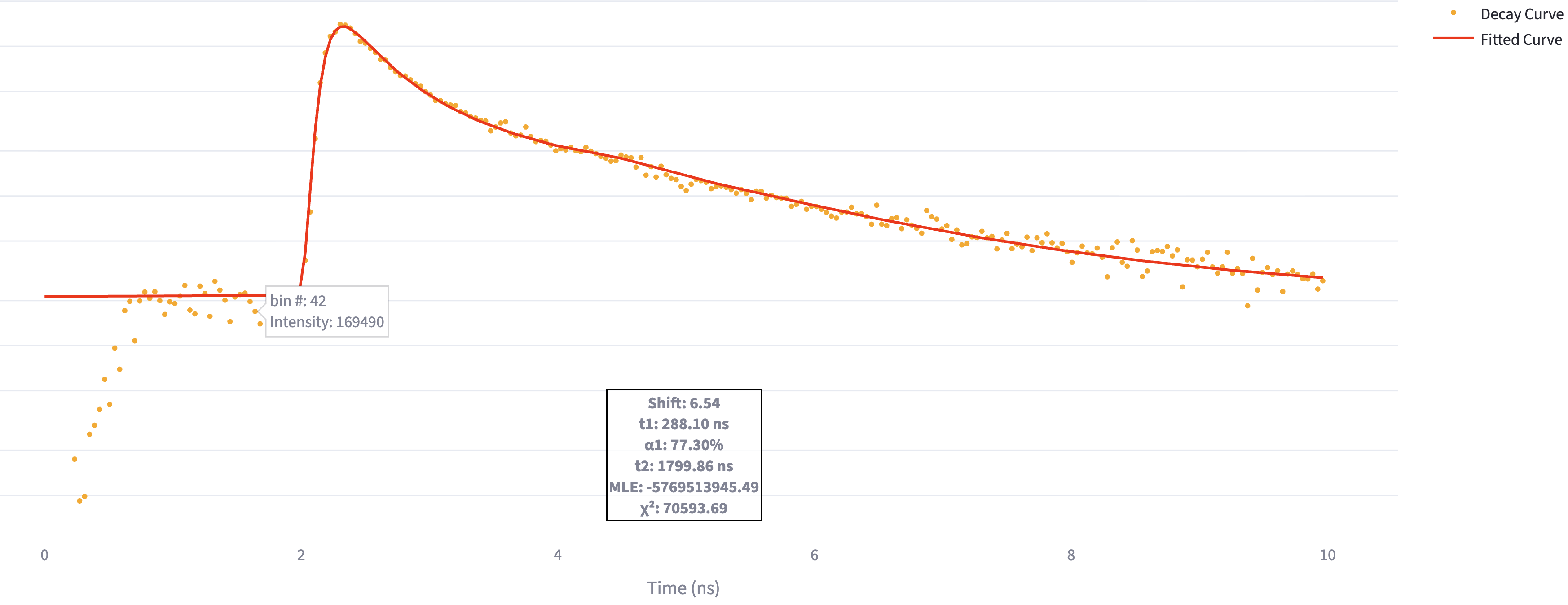
The same Mosaic16 decay after fitting with the 20–240 time gate. The full curve remains visible for inspection.

Metric

Maximum Likelihood Estimation (MLE) estimates the parameters by maximizing the likelihood function, which is the probability of the measured data given the model parameters. A mathematically convenient way to do this is to minimize the negative log-likelihood function:

\[ \text{NLL}(\theta; t_s,t_e) = -\sum_{n=0}^{N-1} \mathbf{1}_{[t_s,t_e)}(t_n)\,\bigl[y_n \log \hat{y}(t_n) - \hat{y}(t_n)\bigr]. \]

\(\mathbf{1}_{[t_s,t_e)}\) is the indicator function that is 1 if \(t_n\) is within the time gates \([t_s, t_e)\), and 0 otherwise. \(y_n\) is the observed count at time \(t_n\), and \(\hat{y}(t_n)\) is the model prediction at \(t_n\).

Weighted Least Squares (WLS) minimizes the squared residuals between the measured curve and the model prediction, with each time bin weighted by the inverse of its expected variance. Because photon counts follow Poisson statistics (variance \(\approx\) mean), the per-bin variance is estimated by the model prediction \(\hat{y}(t_n)\), so each residual is scaled by \(1/\sqrt{\max(\hat{y}(t_n), 1)}\), and the cost minimized is

\[ \text{WLS}(\theta; t_s,t_e) = \sum_{n=0}^{N-1} \mathbf{1}_{[t_s,t_e)}(t_n)\,\frac{\bigl(y_n - \hat{y}(t_n)\bigr)^2}{\max(\hat{y}(t_n), 1)}. \]

This weighting is Pearson’s \(\chi^2\) — the per-bin variance is taken from the model \(\hat{y}(t_n)\) rather than the noisy measured count — which keeps the high-count bins near the decay peak from dominating the fit; the \(\max(\cdot, 1)\) floor avoids division by zero where the model is near zero. The reported reduced chi-square also uses model-based variance, but divides by positive model values without the WLS floor and adjusts for the number of free parameters.

6.4 Fit-Free IRF Calibration

This shift calibration applies to channels with Lifetime fit free selected and calibration method set to IRF, including pre-fitted FLIM channels when phasor features are requested. The fluorescence lifetime standard method instead calibrates phasors during extraction.

Before calculating phasors, the app subtracts the mean signal in the final 10% of each cell’s decay and clips negative values to zero. See fit-free preprocessing.

6.4.1 Shift IRF

It is performed similarly to the fit calibration steps, but in the second step, the shift is not optimized (fitted). It shares the same interface as the fit calibration step, where a scatter plot of the shift values is displayed for each channel, only that the plot is not interactive to show the fit. Instead, it outputs the shift that maximizes the cross-correlation between the IRF and each decay. If Fix the Shift is selected, users can specify the shift value that will be applied to all fields of view. With Fix the Shift cleared, image inputs use their individual FOV shifts; 2D inputs use the median sampled shift within each FOV.

Note

If both Lifetime fit and Lifetime fit free are selected for a raw FLIM channel, the optimized IRF shift from fit calibration is reused for IRF-based phasor extraction. For pre-fitted FLIM, the existing fitted values do not trigger reconvolution fitting; IRF-based phasor extraction uses the cross-correlation shift described above.

The signals of the shifted IRF are deconvolved from the offset-subtracted decay curves using phasor.phasor_divide from the phasorpy package.

6.5 Confirm Calibration

Once satisfied with the fitting options, time gates, and shift values for every required channel, click Confirm calibration for each channel below the channel expanders. The same control confirms QPI background settings when that calibration is included.

After confirmation, the app automatically updates the existing metadata file with the shifts, time gates, fitting options, component counts, and fixed lifetimes. A metadata-save error must be resolved with Retry saving metadata before extraction can run. Continue to the Numerical workflow for extraction and automatic saving.

1.

Warren, S. C. et al. Rapid global fitting of large fluorescence lifetime imaging microscopy datasets. PLoS ONE 8, e70687 (2013).