FLIM Playground

Logo courtesy of Matt Stefely. The yellow dot is a photon sliding down a lifetime decay curve 🛝.1
1 Quick Start

Welcome to the FLIM Playground 🥳🎉🥂! This is an interactive graphical user interface (GUI) that allows you to extract single-cell2 features from fluorescence lifetime imaging microscopy (FLIM), intensity-only, and QPI inputs (Data Extraction) and analyze extracted features or any tabular dataset using a built-in repertoire of methods (Data Analysis).
Several talks have been given about FLIM Playground:
- FLIM Playground @ SPIE 2026: 13 mins
- FLIM Playground @ the Fluorescence Microscopy Summit by Photonics Media: 31 mins
1.1 Try Data Analysis
Load the sample. In the online demo, select Univariate → Feature Comparison. Turn off Use a table from another source and upload this sample dataset. The hosted app starts with this checkbox on; for your own table, leave it on and follow the column review walkthrough.
Compare groups. Select tm under Lifetime fit_nadh, set Color by to
treatment, and Separate by tocell_line. Change a filter or select another measurement to explore the Feature Comparison plot.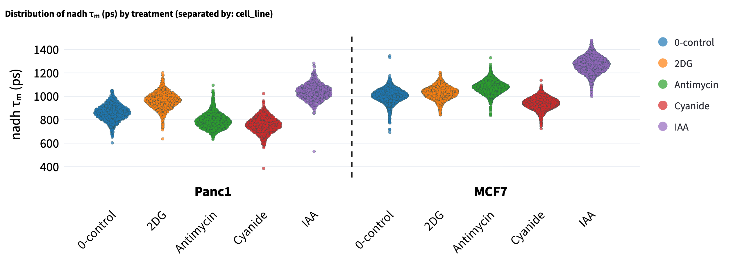
Compare a lifetime measurement across treatments, with a separate section for each cell line. Save the workflow. Below Plot Styling, click Export the entire analysis as a Python script. Keep the original CSV and follow the script workflow to reproduce the plot.

Download a Python script containing the current analysis settings.
- prefer a video walkthrough? See the Data Analysis demo.
1.2 Try Data Extraction locally
Use a local installation for Data Extraction so the app can read input folders and save CSV files on your computer. The Mosaic example contains 25 NADH fields of view (Mosaic01–Mosaic25), with raw FLIM decays, cell masks, and an IRF. It is the same example used in the IRF calibration and time-gate walkthrough.
Download the inputs. Download the Mosaic example ZIP from the FLIM Playground repository and unzip it. Open the extracted
3d_decay_1channelfolder. It contains:- 25
.sdtdecay files, such asMosaic01.sdt. - 25 matching cell masks, such as
Mosaic01_Ch2_summed_cellpose.tiff. nadh_irf.txt, shared by all 25 fields of view.
- 25
Configure the example. In Home, create a profile such as
Mosaic NADH exampleand enter the settings below. Click Update Configuration to save.Setting Value for this example Number of channels / Channel 1 name / Imaging modality 1/NADH/FLIMFLIM input format Decay (3/4D)Extract feature types from NADH Lifetime fitandLifetime fit freeNumber of components 2Laser rate 80MHzFit free calibration method IRFDecay suffix .sdtMask suffix _Ch2_summed_cellpose.tiffIRF suffix nadh_irf.txtUnique cell identifier / FOV column name cell_id/image_nameThe app reads the image dimensions and timing from the SDT files:
512 × 512pixels,256time bins, and a12.5ns decay period. See configuration when adapting this setup to your own inputs.Check the folder. Open Data Extraction → Numerical and enter the full path to the extracted
3d_decay_1channelfolder. Confirm thatMosaic01–Mosaic25report All files found, review any channel assignment and the metadata preview, then click Start calibration. The app automatically saves the metadata in the source folder. See the FOV Metadata reference if a file is missing or duplicated.Calibrate and extract. Continue in Numerical. Keep MLE, two components, Fix the Shift selected, and the initial Start (T1) = 0, End (T2) = 256 gates. Click Optimize for Shifts, then inspect the NADH channel expander. Select
Mosaic16in the shift plot to inspect its decay and fitted curve.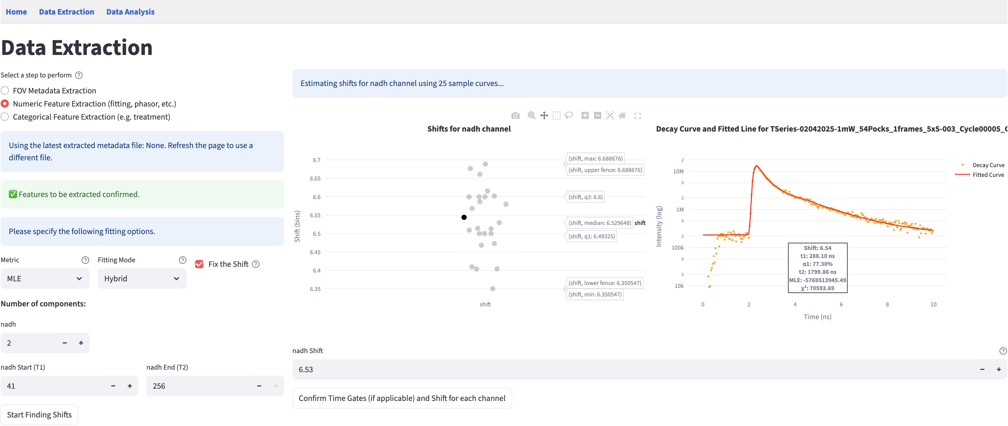
Inspect Mosaic16 in the 25-FOV shift distribution before starting cell-level extraction. The fit is not so good now. Review the shifts and adjust the time gates. Click Confirm calibration for each channel, leave Local selected by default for faster cell-level fitting or change the mode using the mode guidance, then click Start extraction. Confirmation automatically records the calibration, and the app saves the cell-feature CSV in the source folder; see Save Results.
For experiments whose FOV names encode labels such as treatment, follow Categorical Feature Extraction before analysis. Then use the Data Analysis section to visualize and model the extracted features.
For a multi-channel, multi-modal, multi-experiment example, see the Data Extraction demo
1.3 Installation
FLIM Playground is built entirely in Python and is open-source.
For the complete, always-current instructions — per-platform download links, install steps, upgrading, and building from source — see the project README, kept as the single source of truth:
1.4 Introduction
Fluorescence lifetime imaging microscopy (FLIM) measures the time it takes for a fluorescent molecule to emit light (return to the ground state) after being excited by a pulse of light (enter the excited state). It is sensitive to changes in fluorophore microenvironment including, pH, temperature, and conformational changes due to protein-binding and the presence of quenchers1. Coupled with modern automated cell-segmentation methods2, FLIM enables single-cell analyses that can reveal biological heterogeneity.
To acquire FLIM data, a light source—typically a pulsed laser for time-domain methods or a modulated continuous-wave source for frequency-domain methods—is used to excite the fluorophore of interest. The emission is detected using instrumentation capable of resolving fluorescence decay, such as time-correlated single-photon counting (TCSPC), time-gated, or phase/modulation-based detection. In time-domain FLIM, the delay between excitation and photon arrival is measured, and often a histogram is built, with the x-axis representing the delay time and the y-axis representing the number of photons falling into each time bin. Compared to intensity images, FLIM has an additional dimension of time (e.g., 256 time bins per 12.5 nanoseconds).
In frequency-domain FLIM, the phase shift and modulation depth of the emission relative to the excitation are determined.
A diverse set of tools — both open-source and commercial, ranging from libraries to code-free graphical user interfaces (GUIs) — is available to extract and analyze FLIM data, providing alternative methods and therefore flexibility to FLIM researchers. Examples include PhasorPy3, an open-source library for analyzing fluorescence lifetime using the phasor approach; FLUTE4, an open-source GUI for interactive phasor analysis; FLIMPA5, an open-source phasor analysis GUI enabling batch processing, ROI-based quantification, and experiment-level comparison through manual assignment; FLIMLib, an open-source generic curve fitting library that can be used to fit fluorescence lifetime decay data; SPCImage6, a commercial software for fitting and phasor features.
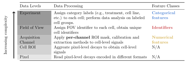
However, while some tools offer code-free interfaces, users still need to write custom code—either to prepare data in the proper format as input, or to further process their outputs for downstream analysis. The fragmentation between tools arises because each focuses on only a subset of data levels: pixel, cell ROI, channel, field of view, and experiment.
- Pixel:
- A single decay curve encoded in vendor-specific file formats (e.g., Becker & Hickl, PicoQuant, etc.)
- Region of Interest (ROI)
- Mask with cell labels
- Channel
- Different fluorophores
- Fluorophore-specific calibration files
- Masks focusing on different parts of the cell (e.g., whole cell, cytoplasm, nucleus, stain, etc.)
- Different feature extraction methods (fitting, phasor, morphology, texture)
- Field of View (FOV)
- Input decay types (e.g., 2D, 3/4D, pixel-level pre-fit lifetime features)
- Experiment
- Different treatments, time points, cell lines, etc., and combinations thereof
An integrated framework should take into account all data levels ■ ■ ■ ■ ■ (•) while maintaining the flexibility to handle various input types (◦). It should provide a level of abstraction to address fragmentation from data levels and input types.
Additionally, the use of FLIM is rapidly evolving, and new methods are being developed all the time. An integrated framework should allow users to choose among alternative methods seamlessly, be the backbone of iterative explorations integral to research, and be ready to incorporate new methods: The provided level of abstraction should address fragmentation from extraction and analysis methods.
Finally, many of the existing tools, including GUI-based software, are not cross-platform, which limits their accessibility. The Installation addresses this last challenge.
A closer parallel to FLIM Playground’s integrated approach is the combination of CellProfiler7, which extracts per-object morphological and texture features, and CellProfiler Analyst8, which ingests these outputs or other feature tables for visualization and statistical analysis. However, FLIM Playground stands apart in that it can extract lifetime features from time-resolved data, alongside morphological and texture features from intensity images. Its general Data Analysis section incorporates FLIM-specific methods (e.g., phasor analysis) and provides statistical models that address additional analysis aspects such as data heterogeneity, in addition to training machine learning classifiers.
1.5 Method
1.5.1 Feature Classes
Tabular data columns can be categorized into three feature classes:
- Identifiers: an optional row identifier for tracking observations; the app supplies row numbers for user tables without one
- Categorical features: conceptually help us group the rows (e.g.,
treatmentwill group the rows into different treatment groups) - Numerical features: quantify the differences/similarities between data groups
Science, from the data perspective, is about closing the conceptual categorical gaps with quantitative measurements.
At data levels, the data are processed to extract the feature classes in Data Extraction, and the classes are used in the Data Analysis section. A user table can also mark columns Ignore; field-of-view labels use the Categorical role. See column roles.
1.5.2 Design
FLIM Playground has two independent sections:
Data Extraction
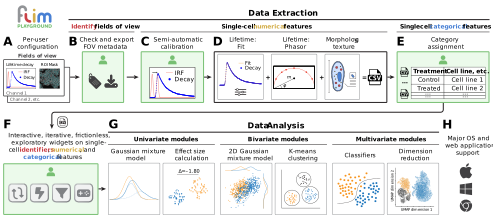
Data Extraction extracts single-cell features from the raw data. It adopts a framework that offers channel-level flexibility in input types and extraction methods without incurring too much overhead for users. The diagram below the Design heading summarizes conceptual components, following the feature classes. In the current interface, metadata preparation, calibration, and numerical extraction run together under Numerical; Categorical combines and labels the resulting tables:
- Data Extraction Configuration (A): allows users to choose among alternative input types and extraction methods (extractors).
- Metadata organization (B), within Numerical: records the field of view identifiers and their configurations
- Numerical Feature Extraction: extracts single-cell numerical features based on user-selected extractors. More extractors can be integrated in the future.
- IRF Calibration (C): estimate shifts for raw lifetime fitting or IRF-based phasor extraction; dye-based calibration is applied during phasor extraction
- Lifetime extractors (D):
- Intensity-based extractors (D):
- QPI dry-mass statistics and spatial texture, with per-channel background correction
- Derived features
- Categorical feature extraction (E): extracts single-cell categorical features and combines experiment-level datasets.
Data Analysis
Data Analysis analyzes features—whether extracted through Data Extraction or by other methods—using visualizations and statistical modeling. It deploys a shared framework (F) built to handle the feature classes across all analysis methods, enabling the same interactive and frictionless exploration experience and allowing new methods to be integrated in the future easily.
- Data Analysis (G) goes in-depth into how FLIM Playground handles the feature classes and Data Analysis Config goes through how users can configure FLIM Playground to analyze datasets that are not extracted by Data Extraction.
Here is the list of analysis methods incorporated into FLIM Playground, grouped by the number of numerical features they take as inputs:
Both sections are built in Python and available in the local app on major operating systems, using a browser interface (H). The hosted app provides Data Analysis only; Data Extraction uses a local installation to read and save files on your computer.
1.5.3 Summary
FLIM Playground resolves these challenges with an interactive code-free graphical user interface (GUI) that spans the full pipeline. It integrates validation checks that guide users at every step, and has a built-in repertoire of analytical methods with interactive widgets that encourage hypothesis-driven, iterative exploration of large datasets. It is built on a modular architecture that enables incorporation of new algorithms in the future.
1.5.4 Citation
FLIM Playground is published in Cell Reports Methods. If it contributed to your research—whether through Data Extraction for single-cell feature generation or through Data Analysis for data exploration, visualization, selection of analysis methods, or hyperparameter tuning (UMAP, clustering, classification, etc.)—please cite this work in your publication. Your citation directly supports us in maintaining and improving it ✨🎈🍾.