19 Classification
A machine learning classifier learns patterns from categorized data and then predicts the category of new, unseen data. This module provides a set of machine learning classifiers and interactive widgets to help users perform classification.
All the classifiers are implemented using scikit-learn and the performance metrics are calculated using sklearn.metrics. A fixed random seed (42) is used for all the classifiers to ensure reproducibility.
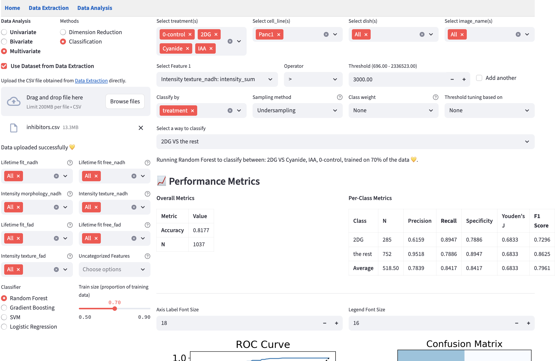 The performance metric plots are cut off in the screenshot. See the performance metrics section for the complete view.
An overview of the pipeline:
- Choose the numerical features on the left.
- The z-score normalization is applied to the features before training if the chosen classifier is
SVMorLogistic Regression, because they are sensitive to feature magnitudes, whileRandom ForestandGradient Boostingare not.
- The z-score normalization is applied to the features before training if the chosen classifier is
- Choose the classifier and train-test split.
- Filter the dataset.
- Choose categorical features to form classes.
- Choose any of the methods to handle class imbalance.
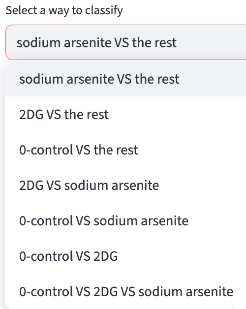
- Choose the classes to be classified.
- Look at the performance metrics, confusion matrix, and ROC curve.
- Iterate over the previous options to improve the performance with regard to the metrics you care about.
19.2 Method-specific Components
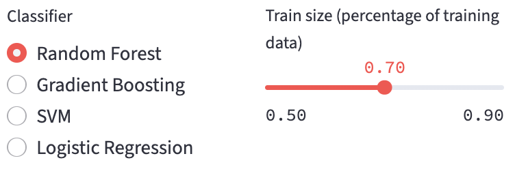
- Choose the classifier and train-test split: the slider controls the proportion of the data used to train the classifier and the rest is used as unseen data to test its generalizability. The following classifiers are available:
Random ForestGradient Boosting- Support Vector Machine (
SVM) Logistic Regression
The train-test split is used to evaluate the generalizability of the classifier. The Validation set is used in hyperparameter tuning. Since the classifiers above do not have a lot of hyperparameters to tune, it does not partition a separate validation set. However, k-fold cross-validation is used in tuning the threshold.
Classify by: TheColor byfrom the visual channels widgets is renamed toClassify byand it is used to form classes based on (a combination of) selected categorical features. Other visual channels are not supported in this method.
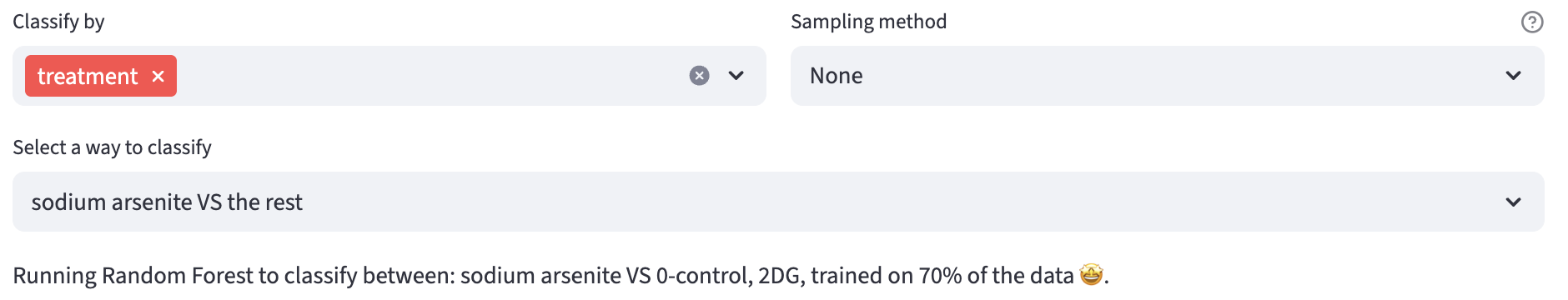
- Choose the classes to be classified: classes are formed based on the combinations of categories of the selected categorical features. In general, it supports binary classification and in general n-way classification where n is the number of classes. If one categorical feature is selected and after filtering has 3 categories, then all possible ways to classify are produced including the three-way classification. Additionally, the
class x vs the restoption is provided for each class.
19.2.1 Classifier Hyperparameters
The classifier hyperparameter panel is organized per classifier with three roles:
Model-Form/Capacity: defines the hypothesis family or expressive power.Regularization: constrains model complexity to reduce overfitting.Optimization: affects training convergence and runtime behavior.
Random Forest
| Param | Role | Effect | Priority |
|---|---|---|---|
n_estimators |
Model-Form/Capacity | More trees increase ensemble capacity; gains usually show diminishing returns after enough trees. | High |
max_depth |
Regularization | Caps tree depth to reduce overfitting; also directly limits capacity. | High |
min_samples_split |
Regularization | Requires more samples before splitting, reducing fragmentation on small partitions. | Medium |
min_samples_leaf |
Regularization | Enforces minimum leaf size, smoothing predictions. | Medium |
max_features |
Regularization | Fewer features per split increase tree diversity and reduce variance/overfitting. | Medium-High |
Gradient Boosting
| Param | Role | Effect | Priority |
|---|---|---|---|
n_estimators |
Model-Form/Capacity | More stages increase additive model capacity; strongly interacts with learning_rate. |
High |
learning_rate |
Regularization | Shrinks each stage contribution; lower values typically need more trees and often generalize better (also affects optimization dynamics). | High |
max_depth |
Regularization | Limits base learner complexity; also limits capacity. | High |
subsample |
Regularization | < 1.0 introduces stochastic boosting, reducing variance and overfitting risk. |
High |
Support Vector Machine (SVM)
| Param | Role | Effect | Priority |
|---|---|---|---|
C |
Regularization | Higher C penalizes training errors more, which usually weakens regularization. |
High |
kernel |
Model-Form/Capacity | Chooses hypothesis family (linear vs non-linear kernels). |
High |
gamma |
Model-Form/Capacity | Controls influence radius of samples for rbf/poly/sigmoid; higher values create tighter boundaries. |
High |
degree |
Model-Form/Capacity | Polynomial order for poly kernel; higher degree increases flexibility. |
Medium-High |
coef0 |
Model-Form/Capacity | Kernel offset for poly/sigmoid, shifting boundary behavior. |
Medium |
tol |
Optimization | Convergence tolerance; mostly affects runtime/termination behavior. | Low |
Logistic Regression
| Param | Role | Effect | Priority |
|---|---|---|---|
regularization |
Regularization | Selects regularization type; available options depend on solver (see table below). Maps to l1_ratio internally. |
High |
C |
Regularization | Inverse regularization strength; higher C means weaker regularization. |
High |
l1_ratio |
Regularization | Balances l1 vs l2 when solver='saga' and regularization='elasticnet'. |
Medium |
fit_intercept |
Regularization | Disabling intercept is a mild structural constraint. | Low |
solver |
Optimization | Optimization algorithm; affects convergence speed and which regularization options are available. | Low-Medium |
max_iter |
Optimization | Iteration budget; too low can stop before convergence. | Low-Medium |
tol |
Optimization | Convergence threshold; mainly runtime-sensitive. | Low |
Regularization options by solver:
| Solver | Available regularization |
|---|---|
lbfgs |
l2, none |
liblinear |
l1, l2 |
newton-cg |
l2, none |
newton-cholesky |
l2, none |
sag |
l2, none |
saga |
l1, l2, elasticnet, none |
19.2.2 Class Imbalance Handling
We provide three options for handling class imbalance (i.e., one or more classes in a dataset have significantly fewer samples than others, which would otherwise cause a classifier to bias toward the majority class). Note: to prevent data leakage, all the methods below are applied to the training set only.
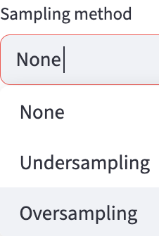
- Sampling methods:
None: stratified random sampling of the data on classification classes, regardless of the class size. It is implemented usingtrain_test_splitfromsklearn.model_selection.Undersampling: All classes are downsampled to the size of the smallest class. It is implemented usingRandomUnderSamplerfromimbalanced-learn.Oversampling: All classes are upsampled to the size of the largest class by randomly duplicating samples from minority classes. It is implemented usingRandomOverSamplerfromimbalanced-learn.
- Class weights:
None: no class weights.Balanced: the class weights are inversely proportional to the class size (support). Note: Gradient Boosting does not support class weights in the scikit-learn implementation, and thus this option is not available for it.
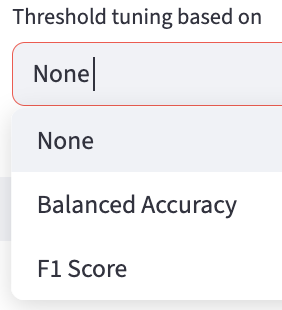
- Threshold tuning: Whereas the previous two options influence the probability estimation part of the classifier, this option adjusts only the decision boundary used to convert predicted probabilities into class labels.
None: no threshold tuning. The default decision is always the class that has the highest predicted probability (in binary, anything above 0.5; in multi-class, the class with the highest predicted probability).Balanced Accuracy: the threshold is set to maximize the balanced accuracy score, which is the unweighted average of each class’s recall (i.e., the minority class’s recall is as important as the majority class’s recall).F1 Score: the threshold is set to maximize the unweighted average of each class’s F1 score.
It treats threshold selection as a separate optimization problem from model training, allowing thresholds to be tuned independently of the underlying classifier’s probability estimates.
K-fold cross-validation for the probability model: The procedure begins by establishing a stratified k-fold cross-validation scheme (default k=5): the dataset is divided into k mutually exclusive subsets, and for each fold, one subset serves as the validation set while the remaining k-1 subsets form the training set.
The probability models are trained separately for each cross-validation fold. This process yields k distinct probability models, each trained on a different subset of the data, along with their corresponding validation set probability predictions that collectively cover all samples exactly once.
Threshold optimization: A single threshold optimization procedure is performed once using all cross-validation folds. The threshold optimization process differs for binary and multi-class classification problems. For binary classification, a single threshold parameter \(\theta \in [0, 1]\) is optimized, where class 1 is predicted when \(P(\text{class } 1 \mid x) \geq \theta\), and class 0 otherwise. For multi-class problems, a threshold vector \(\theta = [\theta_1, \theta_2, \ldots, \theta_k]\) is optimized simultaneously for all \(k\) classes, where thresholds are applied through a normalized probability scheme: predictions are made by selecting the class with the highest normalized probability \(P(\text{class } i \mid x) / (\theta_i + \epsilon)\), where \(\epsilon = 10^{-10}\) prevents division by zero.
The optimization objective function evaluates candidate thresholds by: (1) applying the same threshold(s) on top of the fold-specific probability models to generate prediction classes for the fold-specific validation set, (2) computing the specified evaluation metric (e.g., balanced accuracy, F1-score) between predicted and true labels for each fold, and (3) returning the negative mean cross-validated score across all folds (for minimization using the Nelder-Mead simplex algorithm).
Finally, the optimized threshold(s) are applied on top of the probability model trained on the entire training set to the test set to generate the final predictions.
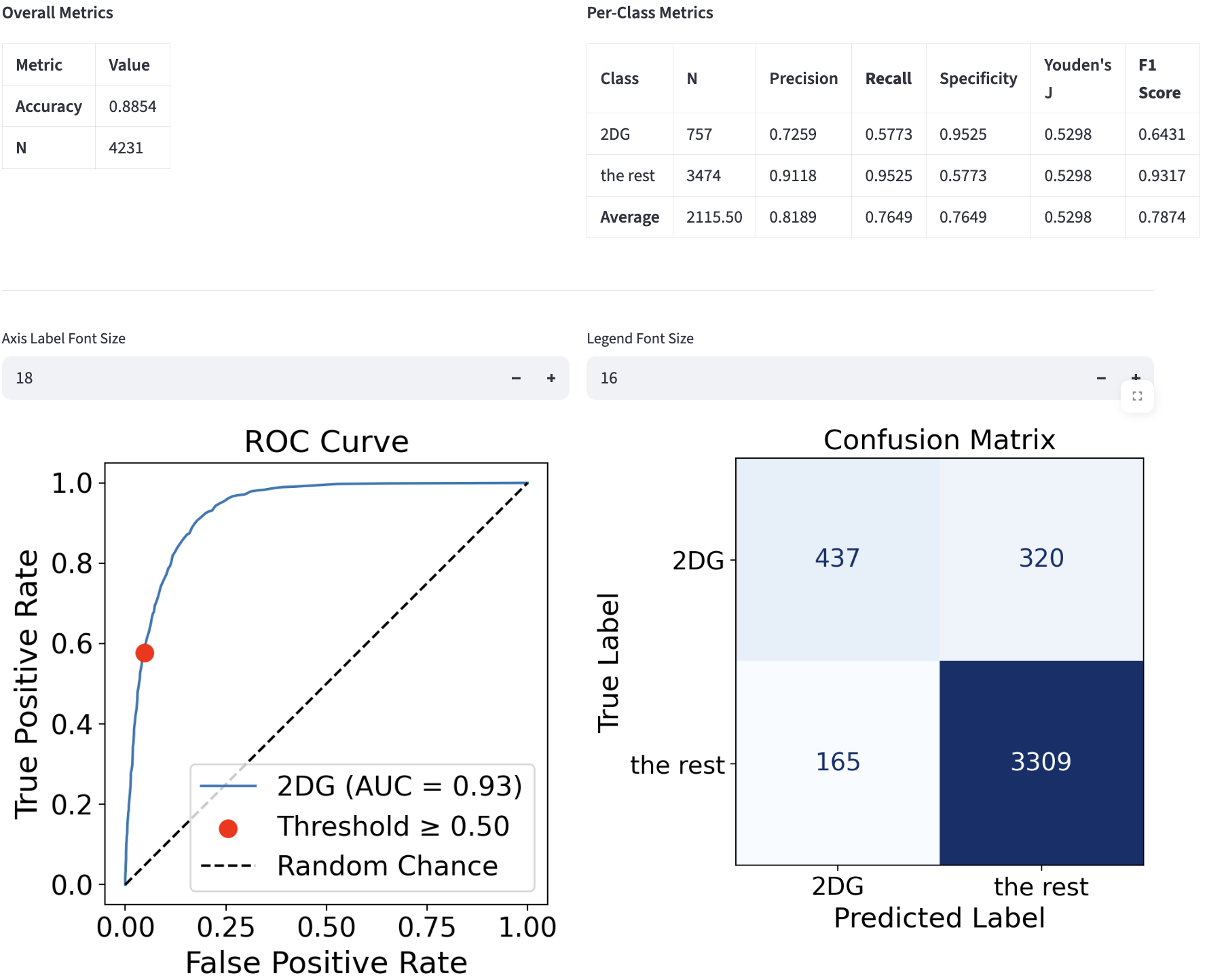
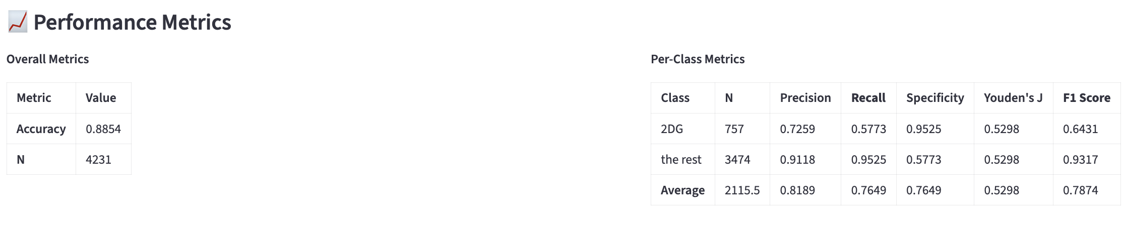
Before threshold tuning:
After threshold tuning based on the balanced accuracy metric:
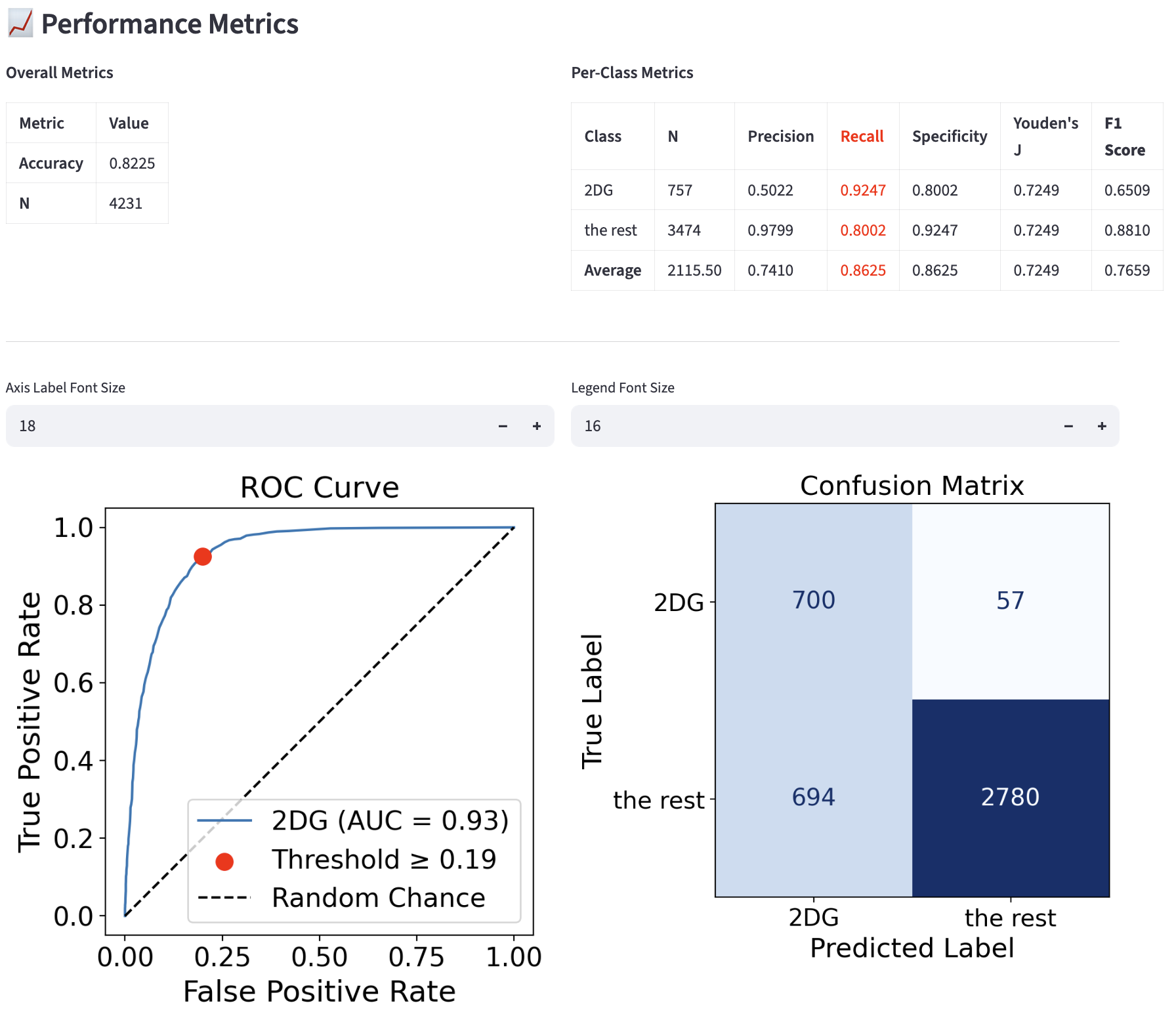
Things to highlight:
- The two ROC curves are the same, because the underlying probability models are the same.
- The annotated operating point in red is “better” after the threshold tuning because it achieves higher Recall (TPR) + Specificity (TNR), as can be seen in the metrics table (the optimized metrics are highlighted in red). The threshold before was 0.5, the default value, and after tuning it was optimized to 0.19. The reduction in thresholds means that the classifier is tuned to be more “confident” at predicting the positive class (2DG), which is the minority class. The effect of this threshold optimization is also visible in the confusion matrix.
- However, all of the above come at the cost of other metrics, such as the overall accuracy (0.89 to 0.82) and average precision (0.82 to 0.74). Select the class imbalance methods/options that maximize the metrics most important to you.
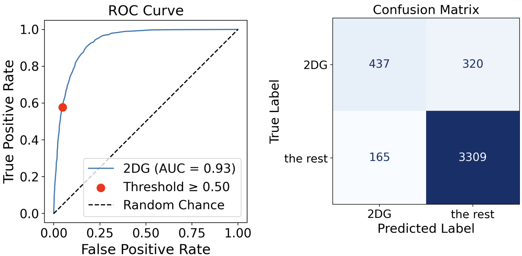
Before sampling:
After sampling (undersampling was used in this case):
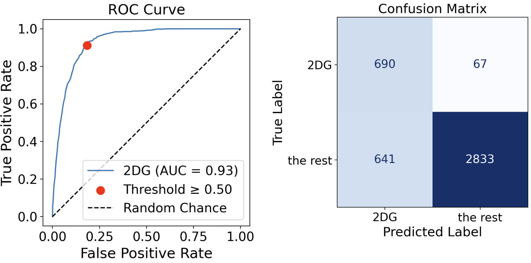
Things to highlight:
- The ROC curve is different, because the underlying probability models are different.
- The thresholds before and after are the same (the default value of 0.5), but the operating points are at different locations and their associated confusion matrices are different.
19.2.3 Confusion Matrix
FLIM Playground evaluates the trained classifier on the held-out test set by converting the predicted probabilities into hard labels using the chosen threshold or by selecting the class with the highest predicted probability. The predictions are then summarized using sklearn.metrics.confusion_matrix. In the binary case, it is represented as:
| Predicted Positive | Predicted Negative | |
|---|---|---|
| Actual Positive | True Positive (TP) – correct hits | False Negative (FN) – missed positives |
| Actual Negative | False Positive (FP) – false alarms | True Negative (TN) – correct rejections |
19.2.4 Performance Metrics
The overall accuracy is calculated as the ratio of the sum of the true positives and true negatives to the sum of all the elements in the confusion matrix (the sum of the diagonal over the sum of all the elements).
- Accuracy: \(\frac{TP + TN}{TP + FP + TN + FN}\)
Other metrics are calculated for each class based on the confusion matrix:
- Precision: \(\frac{TP}{TP + FP}\)
- Recall (Sensitivity): \(\frac{TP}{TP + FN}\)
- Specificity: \(\frac{TN}{TN + FP}\)
- Youden’s Index: \(\text{Sensitivity} + \text{Specificity} - 1\)
- F1 Score: \(\frac{2 \times \text{Precision} \times \text{Recall}}{\text{Precision} + \text{Recall}}\)
The reason that we need metrics in addition to accuracy is because Accuracy is Not Enough. For a visual explanation of metrics, see here. In short, it is all about trade-off.
19.2.5 ROC Curve
Another way to look at the performance of the classifier is to plot the Receiver Operating Characteristic (ROC) curve and its Area Under the Curve (AUC).
Confusion matrix looks at the performance of the classifier at a single threshold, while ROC curve looks at the performance of the classifier at all thresholds (i.e., from 0 to 1).
At the origin (0, 0), the threshold is 1, so the classifier predicts all samples as negative, making the false positive rate \(\text{FPR} = \frac{\text{FP}}{\text{FP} + \text{TN}} = 0\) and the true positive rate \(\text{TPR} = \frac{\text{TP}}{\text{TP} + \text{FN}} = 0\), i.e. the origin. At the point (1, 1), the threshold is 0, so the classifier predicts all samples as positive, making the false positive rate 1 and the true positive rate 1, i.e. the point (1, 1).
AUC summarizes the ROC curve by integrating it from 0 to 1, so it is threshold-free and has a nice interpretation: it is the probability that the classifier assigns a higher score to a randomly chosen positive sample \(X^+\) than to a randomly chosen negative sample \(X^-\).
The ROC curve displays the operating point (FPR, TPR) associated with the confusion matrix on the right.
For a visual explanation, see here.
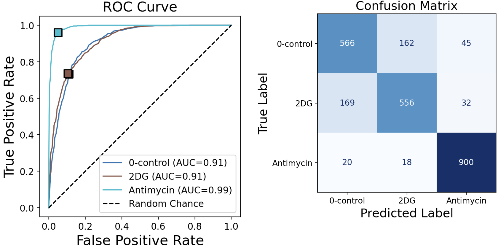
Multi-class ROC Curve
In multi-class classification, each class’s ROC curve is computed as a one-vs-rest binary classification problem. The operating point (FPR, TPR) associated with the confusion matrix is displayed for each class.
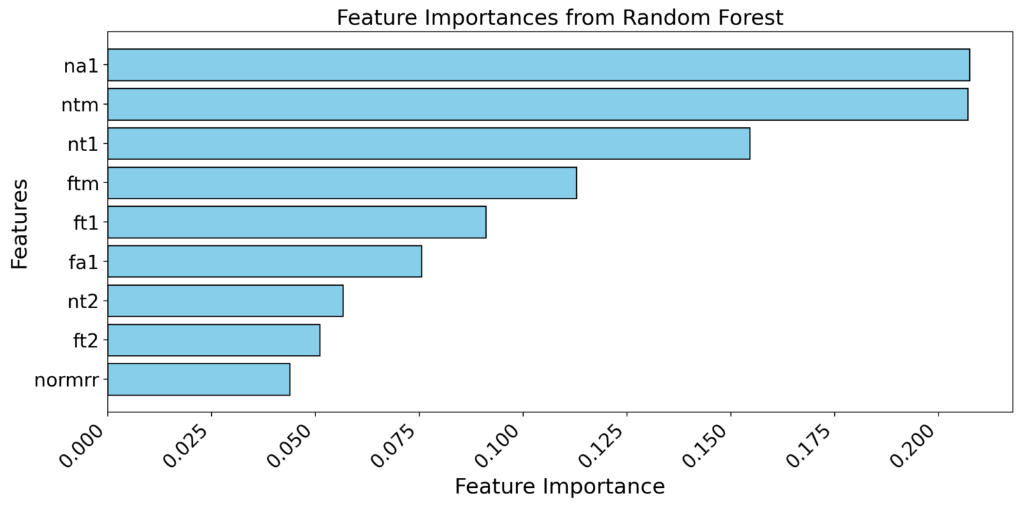
19.2.6 Feature Importance
Random Forest and Gradient Boosting classifiers provide feature importance scores.